Calibrating a SABR volatility cube in Quantra
SABR is the standard model rates desks use to describe the volatility smile, the way swaption implied vols vary with strike, using a handful of parameters. Calibration is the step that fits those parameters to market quotes. This post covers what the model says, what the Volatility Workbench does with it, and, in the style of the curve post, the same calibration reproduced three ways: in the app, as a raw call to the pricing engine, and in QuantLib Python, agreeing to about twelve decimal places.
The model
SABR (stochastic alpha, beta, rho; Hagan et al., 2002) models a forward rate F and its volatility as two correlated random processes:
dF = a F^b dW1
da = v a dW2        with  dW1 dW2 = r dt
The four parameters:
| Parameter | Name | What it does to the smile |
|---|---|---|
| alpha (a) | vol level | Moves the whole smile up and down; roughly the ATM vol |
| beta (b) | backbone | How vol scales with the rate's level; also adds skew |
| rho (r) | correlation | Tilts the smile: negative rho lowers the right wing |
| nu (v) | vol of vol | Curves it: higher nu lifts both wings |
What makes SABR practical rather than just elegant is Hagan's closed-form approximation: given the four parameters, the implied Black vol at any strike is a formula, not a simulation. Pricing an off-grid strike costs nothing, which is why a desk can revalue and bump-risk a whole book against a SABR surface.
Why beta is fixed
Beta and rho do overlapping work: several (beta, rho) pairs produce nearly the same smile, so fitting both is numerically unstable. Hagan et al. recommend choosing beta from prior beliefs about the market rather than fitting it, and market practice for rates settled on fixing it, commonly at 0.5 (see the references). The workbench exposes exactly this: a beta fixed toggle with a value, on by default.
What calibration solves
A swaption surface is a cube: option expiry by underlying swap tenor by strike. At each (expiry, tenor) node the market quotes a smile, a handful of vols at strikes around the ATM forward. Calibration solves, per node:
min over (a, r, v) sum over strikes ( sigma_SABR(K) - sigma_market(K) )^2
optionally weighting each residual by the option's Black vega (the vega weighted option in the workbench), which makes the fit care most about the strikes where vol errors cost the most money. The result is one (alpha, beta, rho, nu) set per node, plus fit diagnostics that tell you how well the model explains your quotes.
In the app
The Volatility Workbench's surface editor, with kind set to SABR Calibrate:
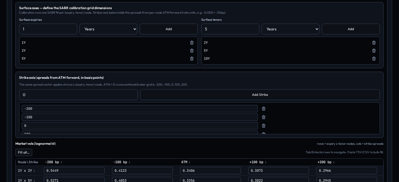 Expiry and tenor axes, the strike axis in basis points, the vols grid, and the SABR options.
- Expiries and tenors define the cube's nodes.
- Strikes are spreads from the ATM forward, in basis points (-200 to +200 in this example). This matches how the market quotes smiles and how QuantLib's cube API works: the same spread vector applies at every node, and each node centers it on its own forward. A 0 column (true ATM) is not required; the ATM vol is interpolated from your grid.
- The vols grid has one row per (expiry, tenor) node and one column per strike; values are absolute market vols. One paste fills the whole cube.
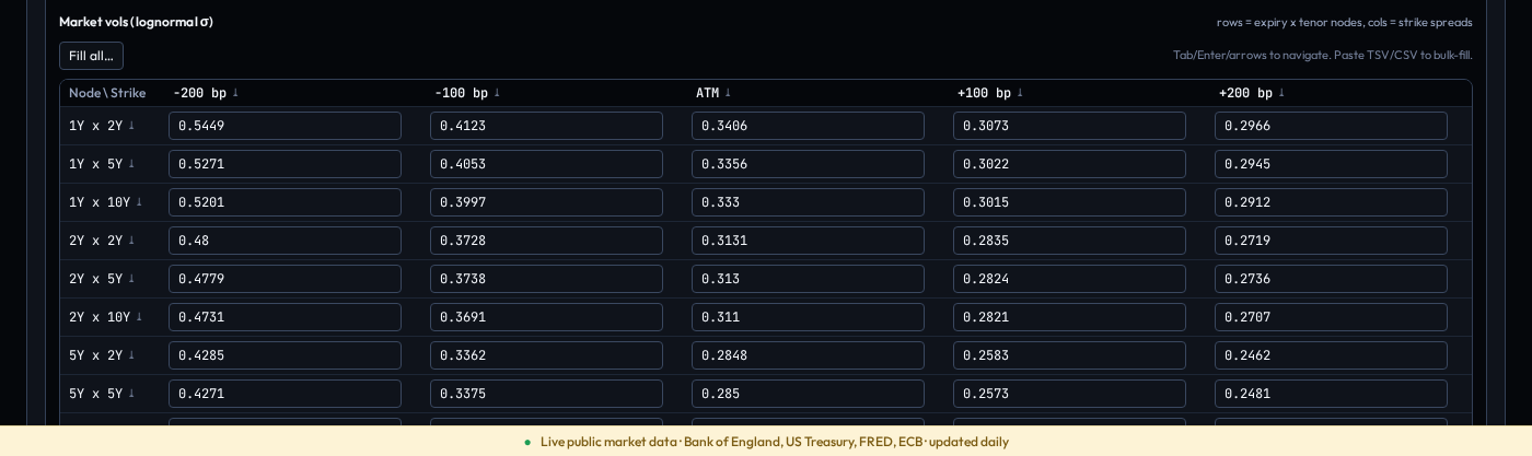 One row per node, one column per strike spread.
Where the vols come from: you type or paste them. There is no public free source of swaption vol surfaces; that is broker and vendor data. The market data import can load your own series into the catalog, but the grid itself is entered inline.
Pressing Calibrate sends the cube, with the discounting and forwarding curves, to the engine and renders the diagnostics:
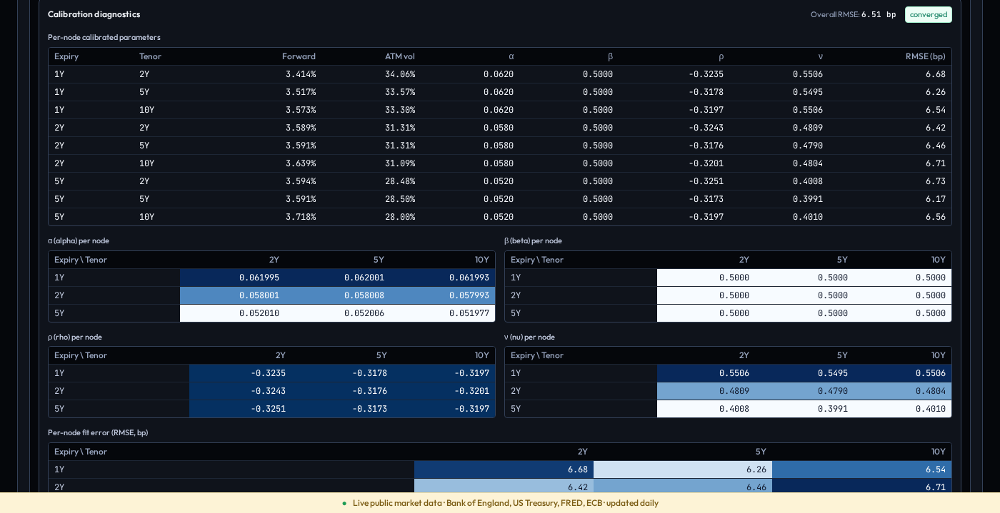 Per-node parameters, fit error per node in basis points, convergence, and parameter heatmaps.
There is no public source of swaption vols, so the demo's quotes are invented, in a way that makes the calibration checkable. They were built in two steps. First, pick SABR parameters for each expiry row and compute the smiles from Hagan's formula: alpha 6.2%, 5.8% and 5.2% for the 1Y, 2Y and 5Y rows, rho -0.32, nu 0.55, 0.48 and 0.40. The resulting smiles are skewed the way rates smiles are: at the 1Y by 2Y node the quote 200bp below the ATM is about 54%, against about 30% at 200bp above it. Second, add a few basis points of noise, so the data does not sit exactly on the model; real quotes never do. Because the generating parameters are known, the result can be verified: the fitted alpha steps down 0.062, 0.058, 0.052 by expiry exactly as chosen, rho comes back within 0.01 of -0.32 at every node, and the injected noise reappears as an honest 6.5bp overall RMSE, converged, with no warnings.
When the data is not perfectly SABR shaped, the diagnostics say so instead of hiding it: each node reports its RMSE, and nodes fitting worse than a threshold produce explicit warnings. You will see that in the example below, on purpose.
Calibration turns the raw quotes into a surface, and a surface can be drawn. Pressing Sample on the calibrated cube evaluates it on a dense expiry by tenor grid and renders the matrix and the 3D view:
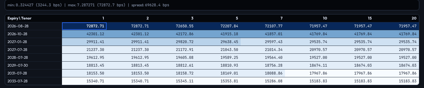 The calibrated cube sampled on an expiry by tenor grid, in basis points.
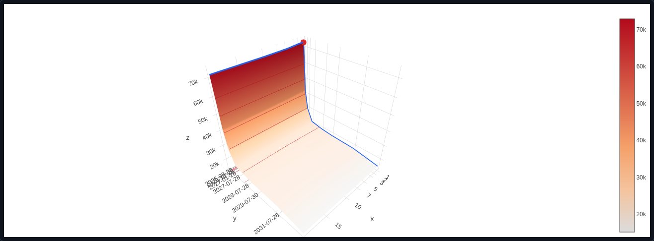 The same calibrated surface in 3D.
The whole example lives on the public demo: open EUR SABR cube in the Volatility Workbench, press Calibrate to reproduce the parameters above, then press Sample to draw the surface they define.
The same calibration three ways
The setup: a 2 by 2 cube (expiries 1Y and 5Y, tenors 2Y and 5Y), five strikes from -200bp to +200bp, a deliberately symmetric smile at every node (for example 24%, 22%, 21%, 22%, 24% at the 1Y2Y node), flat discount and forwarding curves at 2% and 2.5%, beta fixed at 0.5. A symmetric smile is not something a beta 0.5 SABR can fit exactly, which is the point: it exercises the honest-diagnostics path.
This is the call the app makes, expressed against the engine's public JSON API (quantraserver). The curves are two flat zero-rate value curves of the kind the curve post ends with; the index and swap index carry their full conventions, as engine 0.5.0 requires:
POST https://api.quantra.io/calibrate-swaption-vol
{
  "pricing": {
    "as_of_date": "2026-07-24",
    "rates": {
      "curves": [
        {"id": "DISC", "...": "flat 2% InterpolatedZero value curve"},
        {"id": "FWD",  "...": "flat 2.5% InterpolatedZero value curve"}
      ],
      "indices": [{
        "id": "forwarding_index", "index_type": "Ibor",
        "tenor": {"n": 6, "unit": "Months"}, "fixing_days": 2,
        "calendar": "TARGET", "business_day_convention": "ModifiedFollowing",
        "day_counter": "Actual360", "end_of_month": false, "currency": "EUR"
      }],
      "swap_indices": [{
        "id": "EUR_SWAP_6M", "kind": "IborSwapIndex", "spot_days": 2,
        "calendar": "TARGET", "business_day_convention": "ModifiedFollowing",
        "end_of_month": false, "float_index_id": "forwarding_index",
        "fixed_leg": {"fixed_frequency": "Annual",
          "fixed_day_counter": "Thirty360", "fixed_calendar": "TARGET",
          "fixed_bdc": "ModifiedFollowing", "fixed_term_bdc": "ModifiedFollowing",
          "fixed_date_rule": "Forward", "fixed_eom": false},
        "float_leg": {"float_tenor": {"n": 6, "unit": "Months"},
          "float_calendar": "TARGET", "float_bdc": "ModifiedFollowing",
          "float_term_bdc": "ModifiedFollowing", "float_date_rule": "Forward",
          "float_eom": false}
      }]
    },
    "volatility": {
      "vol_surfaces": [{
        "id": "EUR-SABR",
        "payload_type": "SwaptionVolSpec",
        "payload": {
          "swap_index_id": "EUR_SWAP_6M",
          "payload_type": "SwaptionSabrCalibrateSpec",
          "payload": {
            "base": {"reference_date": "2026-07-24", "calendar": "TARGET",
              "business_day_convention": "ModifiedFollowing",
              "day_counter": "Actual365Fixed", "volatility_type": "Lognormal",
              "shape": "SabrCalibrate"},
            "expiries": [{"n": 1, "unit": "Years"}, {"n": 5, "unit": "Years"}],
            "tenors":   [{"n": 2, "unit": "Years"}, {"n": 5, "unit": "Years"}],
            "strikes": [-0.02, -0.01, 0.0, 0.01, 0.02],
            "vols": {"n_1": 2, "n_2": 2, "n_3": 5, "values": [
              0.24, 0.22, 0.21, 0.22, 0.24,
              0.23, 0.21, 0.20, 0.21, 0.23,
              0.22, 0.20, 0.19, 0.20, 0.22,
              0.21, 0.19, 0.18, 0.19, 0.21]},
            "beta_fixed": true, "beta_value": 0.5,
            "vega_weighted_smile_fit": false
          }
        }
      }]
    }
  },
  "vol_id": "EUR-SABR",
  "discounting_curve_id": "DISC",
  "forwarding_curve_id": "FWD"
}
The engine answers with the calibrated cube:
| Node | Forward | ATM vol | alpha | beta | rho | nu | RMSE |
|---|---|---|---|---|---|---|---|
| 1Y x 2Y | 2.5318% | 21.83% | 0.034546 | 0.5 | 0.7235 | 0.2044 | 74.5 bp |
| 1Y x 5Y | 2.5311% | 20.82% | 0.032966 | 0.5 | 0.7182 | 0.1990 | 74.4 bp |
| 5Y x 2Y | 2.5319% | 19.83% | 0.030875 | 0.5 | 0.7206 | 0.1902 | 74.8 bp |
| 5Y x 5Y | 2.5311% | 18.82% | 0.029351 | 0.5 | 0.7143 | 0.1851 | 74.6 bp |
plus four warnings, one per node, naming the RMSE and the threshold it exceeds. That is the correct answer for this input: a symmetric smile with beta 0.5 has no exact SABR fit, and the calibrator returns the best one and tells you how far off it is rather than pretending.
And the equivalent QuantLib Python, using the same guesses and flags the engine uses internally (initial guess alpha 0.04, nu 0.4, rho 0, beta fixed at 0.5, optimizer left at QuantLib defaults on both sides):
import QuantLib as ql

as_of = ql.Date(24, 7, 2026)
ql.Settings.instance().evaluationDate = as_of

disc = ql.YieldTermStructureHandle(ql.FlatForward(as_of, 0.02, ql.Actual365Fixed()))
fwd = ql.YieldTermStructureHandle(ql.FlatForward(as_of, 0.025, ql.Actual365Fixed()))

ibor = ql.IborIndex("Euribor", ql.Period("6M"), 2, ql.EURCurrency(), ql.TARGET(),
                    ql.ModifiedFollowing, False, ql.Actual360(), fwd)
swap_index = ql.SwapIndex("EUR_SWAP_6M", ql.Period("2Y"), 2, ql.EURCurrency(),
                          ql.TARGET(), ql.Period("1Y"), ql.ModifiedFollowing,
                          ql.Thirty360(ql.Thirty360.BondBasis), ibor, disc)

expiries = [ql.Period("1Y"), ql.Period("5Y")]
tenors = [ql.Period("2Y"), ql.Period("5Y")]
spreads = [-0.02, -0.01, 0.0, 0.01, 0.02]
vols = [[0.24, 0.22, 0.21, 0.22, 0.24], [0.23, 0.21, 0.20, 0.21, 0.23],
        [0.22, 0.20, 0.19, 0.20, 0.22], [0.21, 0.19, 0.18, 0.19, 0.21]]

atm = ql.Matrix(2, 2)
for i in range(2):
    for j in range(2):
        atm[i][j] = vols[i * 2 + j][2]          # ATM = the 0-spread column

atm_structure = ql.SwaptionVolatilityMatrix(
    ql.TARGET(), ql.ModifiedFollowing, expiries, tenors, atm,
    ql.Actual365Fixed(), False, ql.ShiftedLognormal)

spread_handles = [[ql.QuoteHandle(ql.SimpleQuote(v - node[2])) for v in node]
                  for node in vols]
guesses = [[ql.QuoteHandle(ql.SimpleQuote(g)) for g in (0.04, 0.5, 0.4, 0.0)]
           for _ in range(4)]

cube = ql.SabrSwaptionVolatilityCube(
    ql.SwaptionVolatilityStructureHandle(atm_structure),
    expiries, tenors, spreads, spread_handles,
    swap_index, swap_index, False,          # vegaWeightedSmileFit
    guesses, [False, True, False, False],   # beta fixed
    False)                                  # isAtmCalibrated

params = cube.sparseSabrParameters()        # rows: alpha, beta, nu, rho, ...
Running both and diffing every reported quantity across all four nodes:
| Quantity | Max abs difference |
|---|---|
| alpha | 2.9e-14 |
| beta | 0 (exact) |
| rho | 2.3e-12 |
| nu | 7.3e-13 |
| forward | 3.3e-16 |
| per-node RMSE | 1.9e-16 |
| fitted vol per strike | 3.2e-13 |
No tuning on either side; the residual differences are floating-point noise
between a C++ build and the Python wheel inside the Levenberg-Marquardt
iterations. The app, the engine API, and QuantLib Python are computing the same
thing, because they are the same thing: the engine wraps QuantLib's
SabrSwaptionVolatilityCube and the app is a front end for the engine.
To run it yourself, use the engine standalone from quantraserver, or try the live demo.
References
- Hagan, Kumar, Lesniewski, Woodward, Managing Smile Risk, Wilmott Magazine, September 2002. The SABR paper: the model, the closed-form vol expansion, and the hedging argument.
- Peter Caspers, Fooling around with QuantLib: SABR. Notes from a QuantLib maintainer, including shifted SABR for negative rates.
- QuantLib term structure and volatility documentation,
covering
SabrSwaptionVolatilityCubeand the smile section classes used here. - Wikipedia, SABR volatility model, including the discussion of fixing beta and estimating it from log-log regression of ATM vols against forwards.