Bootstrapping yield curves in Quantra
Most products in Quantra price against a yield curve, so curve construction is where pricing starts. This post walks through the curve builder end to end: what a curve definition is, the quantitative choices and what they mean in QuantLib terms, every instrument type you can put on a curve, and, at the end, the same live curve reproduced three ways: in the app, as a raw call to the pricing engine, and in thirty lines of QuantLib Python, matching to every printed digit.
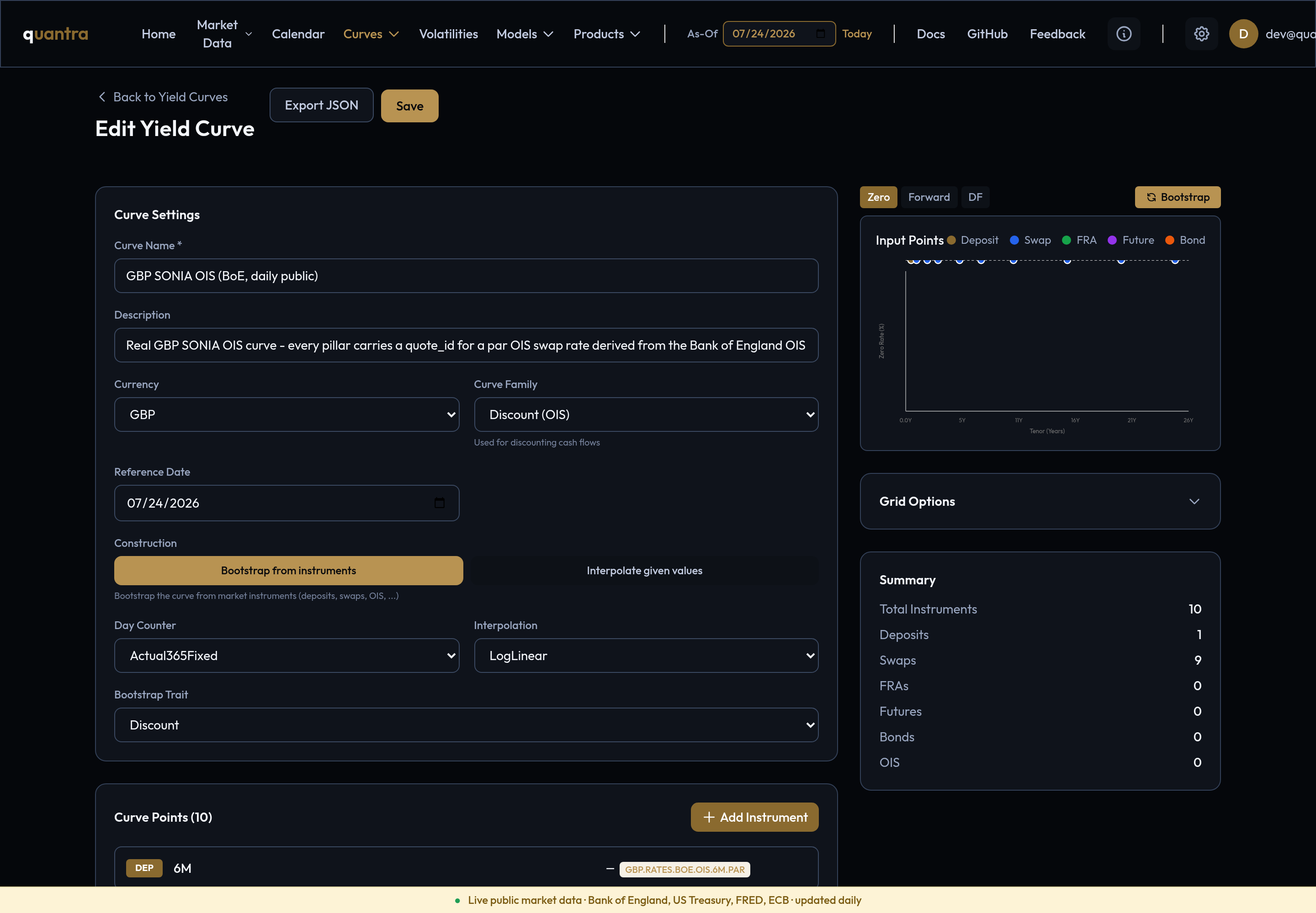 The curve builder with the live GBP SONIA OIS curve: settings and instruments on the left, the bootstrapped result on the right.
What "building a curve" means here
A curve in Quantra is a definition, not a table of numbers: a set of market instruments (deposits, swaps, OIS, and so on), each carrying a quote and its own market conventions, plus the settings that tell the engine how to turn those instruments into a discount function. Nothing is computed in the browser; the definition is handed to the pricing engine, a C++ server built on QuantLib, which bootstraps the curve and returns it. The preview and real pricing run through the same path, so a curve that previews is a curve that prices.
Bootstrapping itself is the classic procedure: find the one curve that reprices every input instrument to its quoted market level simultaneously. Each instrument pins the curve down out to its maturity, so a curve is assembled from the shortest deposit out to the longest swap, and QuantLib solves the whole system iteratively. QuantLib is the brain here, not Quantra; Luigi Ballabio's notes on bootstrapping an interest-rate curve describe the machinery in detail.
Curve settings
The top panel holds the identity and the quantitative choices:
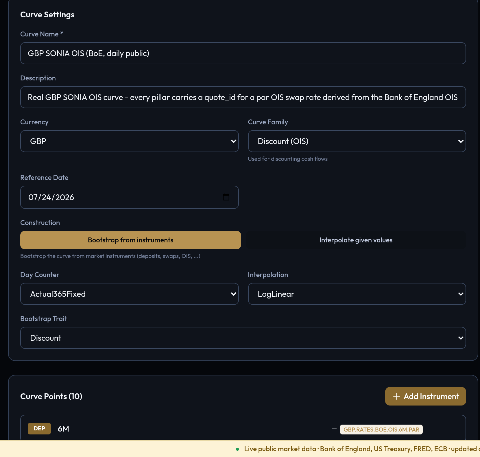 Currency, reference date, day counter, and the two choices that define the mathematics: interpolation and trait.
- Currency: the curve's currency, used to match it against trades and indices.
- Curve family: the curve's role. A discount (OIS) curve discounts cash flows, a forward curve projects an index, plus basis and inflation. Curve sets use this to know which slot a curve can fill.
- Reference date: day zero of the curve, the date all discount factors are measured from. Instrument schedules are generated forward from here.
- Day counter: how the curve converts dates to year fractions when it quotes you a zero rate (Actual/360, Actual/365 Fixed, 30/360 variants, Actual/Actual flavours).
- Interpolation and Bootstrap trait: the mathematics, covered next.
Traits and interpolators: what gets built
QuantLib has two distinct families of yield curves, and the trait dropdown spans both.
Family one: bootstrapped curves. PiecewiseYieldCurve<Trait, Interpolator> is the
template QuantLib uses to bootstrap a curve from market instruments. The trait
chooses which quantity the bootstrapper solves for and stores at each instrument
maturity (each "pillar"); the interpolator chooses how that quantity behaves
between pillars. Three traits belong to this family:
| Trait | QuantLib type | The curve is built on |
|---|---|---|
Discount |
Discount |
Discount factors P(0,T) |
ZeroRate |
ZeroYield |
Continuously-compounded zero rates |
FwdRate |
ForwardRate |
Instantaneous forward rates |
Family two: interpolated curves. QuantLib also has curves that skip bootstrapping
entirely: InterpolatedZeroCurve, InterpolatedDiscountCurve,
InterpolatedForwardCurve. You hand them known values directly (dates and zero rates,
for instance) and they just interpolate through them. No instruments, no solving. The
InterpolatedZero, InterpolatedDiscount and InterpolatedFwd entries in the trait
dropdown mirror this family.
The trait is the explicit selector between the two families, and the engine
validates it against the points you send: the three bootstrap traits require
instrument helpers, while InterpolatedZero, InterpolatedDiscount and
InterpolatedFwd require the corresponding value points (a zero rate, a discount
factor, or an instantaneous forward at each pillar). A mismatch, or a mix of point
kinds in one curve, is rejected with a clear error. All three interpolated families
are implemented as of engine 0.5.0.
The five interpolators apply to both families:
| Interpolator | Between pillars |
|---|---|
Linear |
Straight lines on the trait quantity |
LogLinear |
Straight lines on its logarithm |
LogCubic |
Monotonic cubic spline on the logarithm (QuantLib's MonotonicLogCubic) |
BackwardFlat |
Piecewise constant, each value held backward |
ForwardFlat |
Piecewise constant, each value held forward |
Both families are covered in depth in Ballabio's yield term structures and bootstrapping chapters.
The combination matters more than either choice alone:
Discount+LogLinearis the most common choice. Log-linear interpolation of discount factors is equivalent to piecewise-constant instantaneous forward rates between pillars: simple, fast, and discount factors stay positive and decreasing if the inputs are sane. Its known cosmetic flaw is that the forward curve is a step function.FwdRate+BackwardFlatbuilds the piecewise-flat forward curve directly, essentially the same object approached from the other side.ZeroRate+Lineargives the smooth-looking zero curve people expect on a chart, at the cost of small oscillations in forwards.Discount+LogCubicproduces smooth forwards; the monotonic variant tames the overshooting a plain cubic spline exhibits around sharp corners of the curve.
Instruments: the points on the curve
Each row in the instruments list is one market instrument contributing one pillar. Seven types are supported:
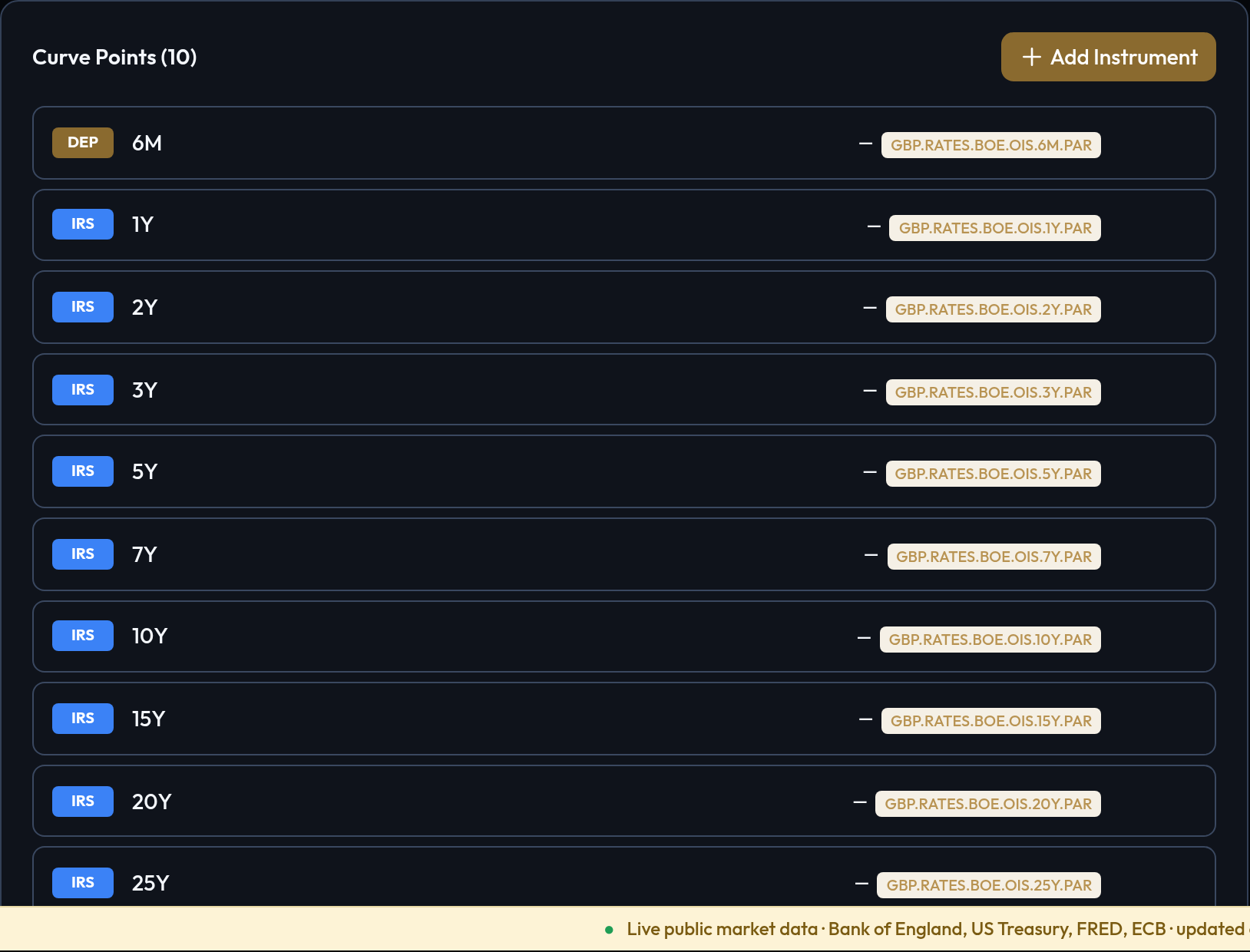 Each instrument covers a segment of maturity space; together they span the curve.
| Type | Typical segment | What it pins down |
|---|---|---|
| Deposit | Overnight to ~1Y | Simple interbank lending rate for one period |
| FRA | Months 1–2 out to ~2Y | Forward rate between two future dates (e.g. 3×6) |
| Future | ~3M to ~2Y | Exchange-traded forward rate, quoted as 100 − rate, with an optional convexity adjustment |
| Swap | 1Y out to 50Y | Par rate of a fixed-vs-floating interest rate swap |
| OIS | Overnight out to 50Y | Par rate of a fixed-vs-overnight-compounded swap, by tenor |
| Dated OIS | Custom | An OIS between two explicit dates rather than a tenor, useful around central-bank meeting dates |
| Bond | Anywhere | A fixed-rate bond quoted by clean price, with its full coupon schedule |
A classic single-curve setup is deposits for the short end, futures or FRAs for the
middle, and swaps from two years out. The live GBP curve on the
public demo is one 6M deposit plus nine swap helpers from 1Y
to 25Y, every pillar referencing a Bank of England SONIA OIS par-rate series
(GBP.RATES.BOE.OIS.5Y.PAR and friends) refreshed daily.
Adding an instrument
Add Instrument opens the editor. The form adapts to the instrument type; what stays constant is the structure: a quote, a tenor or date range, and the market conventions of that instrument.
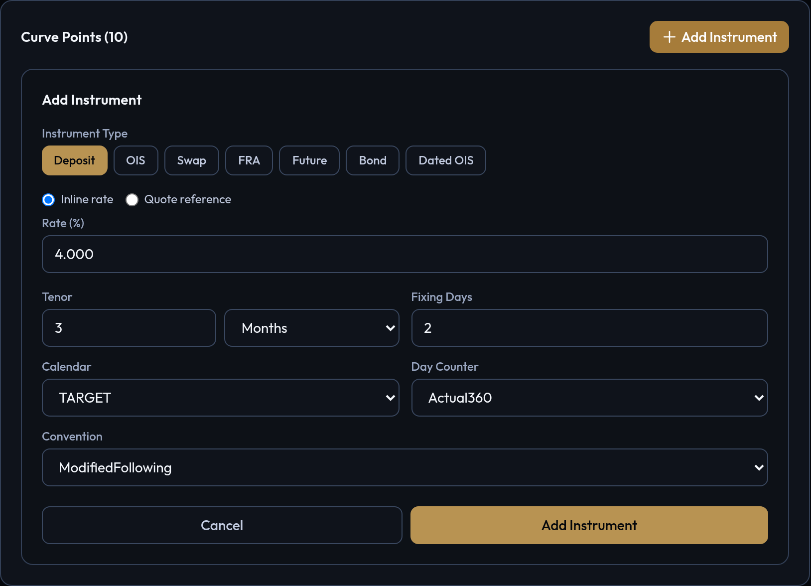 The deposit form: quote source at the top, then tenor, fixing days, and the instrument's own conventions. Selecting another type swaps the fields below.
Every instrument carries its own conventions rather than inheriting them from the curve, because that is how the market quotes: a EUR 6M deposit and a EUR 10Y swap fixed leg do not share a day counter. Concretely:
- Deposit: tenor, fixing days, calendar, business day convention, day counter.
- FRA: months to start and months to end (a 3×6 FRA is
3and6), fixing days, calendar, convention, day counter. - Future: start date, length in months, price, optional convexity adjustment, calendar, convention, day counter.
- Swap: tenor, the floating index (a reference to a saved index definition, e.g. EURIBOR 6M, which brings its own tenor, calendar and fixing rules), fixed leg frequency, convention and day counter, an optional spread, and optional forward start days.
- OIS: tenor, the overnight index (ESTR, SOFR, SONIA), settlement days, fixed leg frequency, convention and day counter.
- Dated OIS: explicit start and end dates instead of a tenor, otherwise as OIS.
- Bond: clean price, face amount, coupon rate, redemption, issue date, and the full coupon schedule (effective and termination dates, frequency, calendar, both conventions, date generation rule, end-of-month flag).
Where the quote comes from: inline vs market data
At the top of the editor every instrument offers two quote sources:
- Inline rate: you type the number (in percent, as quoted). The rate is frozen into the curve definition. Good for experiments, textbook examples, and reproducing a curve from a paper.
- Quote reference: you pick a series from the market-data catalog (for example
GBP.RATES.BOE.OIS.5Y.PAR). The definition stores the reference, and the value is resolved at pricing time, as of the As-Of date, with previous-business-day semantics: the most recent published value on or before that date. This is what makes a curve live: the same definition prices on today's data today and yesterday's data yesterday, and re-pricing a historical date replays the data that was current then.
If a quote reference cannot be resolved at the requested As-Of, the bootstrap does not guess: you get an error listing exactly which series and date failed.
Dependencies: multi-curve setups
Swap and OIS helpers accept an optional discount curve dependency. This is the standard post-2008 dual-curve construction: the swap's floating leg forecasts off the curve being built, while its cash flows discount on a separate (typically OIS) curve. Build the discount curve first, then reference it from the projection curve's swap helpers. The floating index on a swap helper is itself a reference to a saved index definition, so conventions live in one place and every curve and trade that uses EURIBOR 6M agrees on what EURIBOR 6M is.
Building a curve from values instead
Sometimes you already have the curve: a zero curve a central bank publishes, a discount grid exported from a risk system, a forward path from a model. The builder's Construction toggle switches from bootstrapping to interpolating given values.
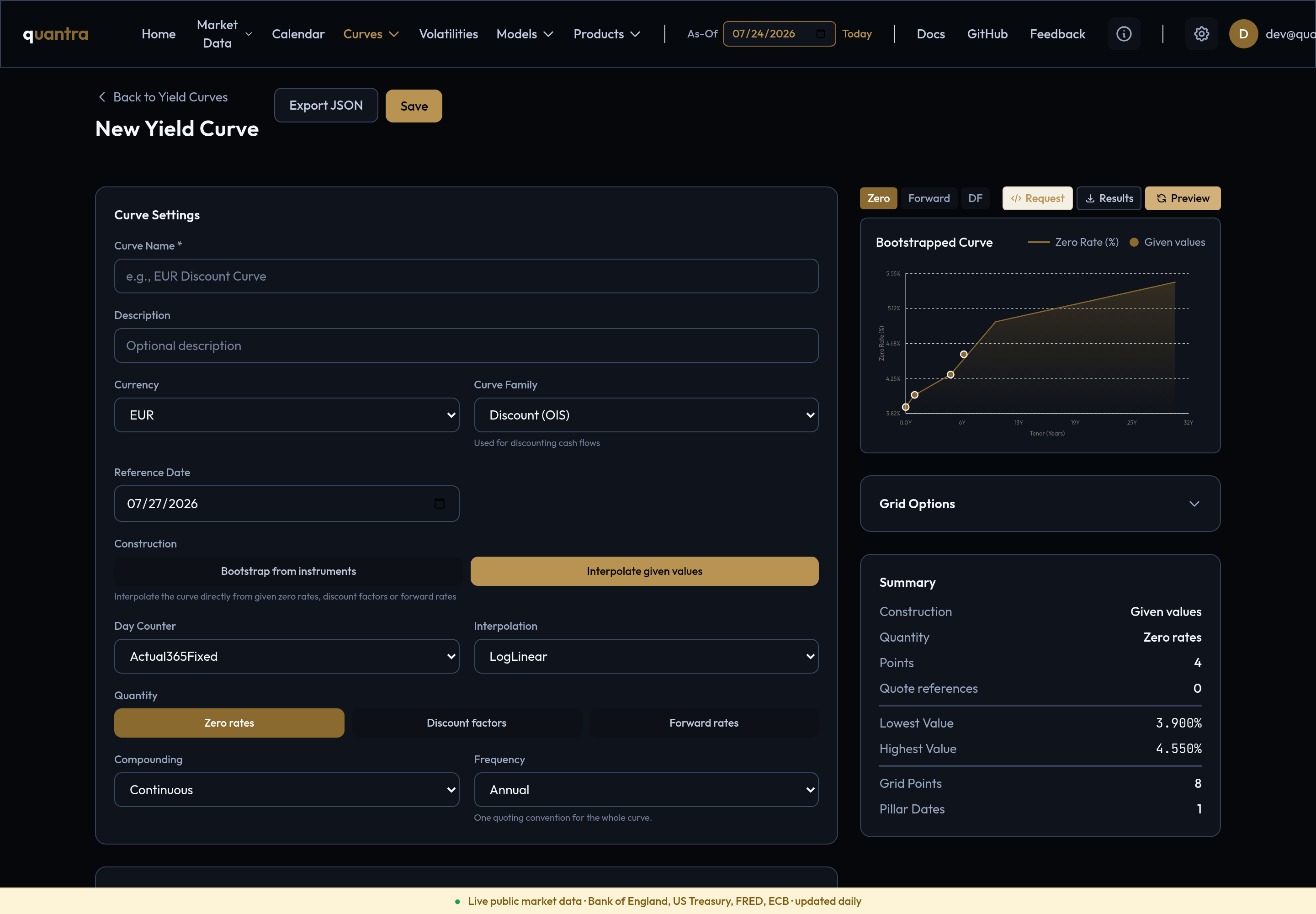 Values mode: pick the quantity, the interpolator, and one quoting convention for the whole curve.
- Pick the quantity you have: zero rates, discount factors, or forward rates. This is exactly the choice between the three interpolated families above: which column of the table the curve is, with everything else derived.
- The first pillar is pinned at the curve's start (its reference date), because the engine anchors an interpolated curve at its first point. For discount factors that value is fixed at 1.0 by definition; for zeros and forwards it is the short end of the curve, and you enter it.
- Every other row is a maturity, as a tenor or an explicit date, plus a value: entered inline or referencing a market-data series resolved at the As-Of date, exactly like instrument quotes. Rows keep themselves sorted by date.
- Paste table accepts a two-column block copied from anywhere: tenors or dates on the left, values on the right.
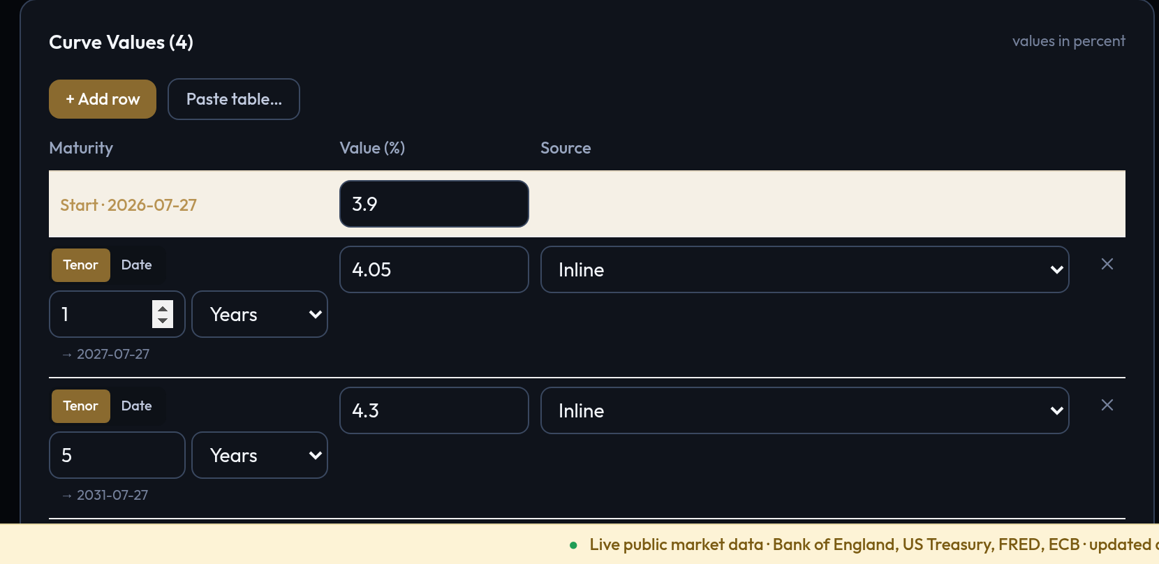 The values table: a pinned start row, then one row per pillar, tenor or date.
A value curve saves, versions and prices exactly like a bootstrapped one: put it in a curve set and a swap will discount on it.
The result: chart, grid, summary
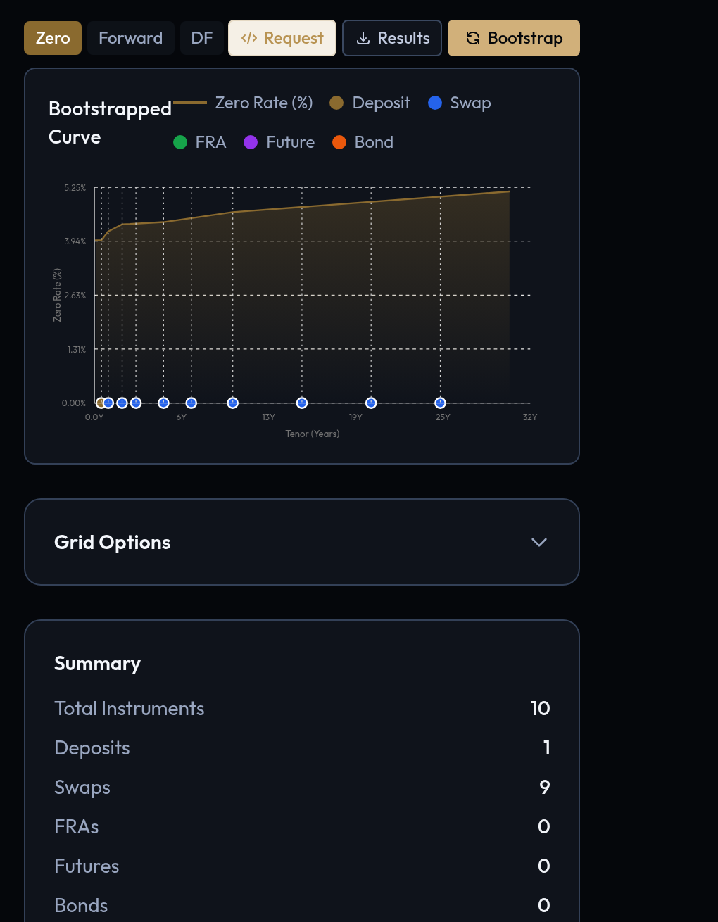 The bootstrapped GBP SONIA curve: zero rates against maturity, input instruments marked along the axis.
- The chart plots the bootstrapped curve against maturity, with markers at the input instruments. Three toggles switch the quantity displayed: Zero (zero rates in percent), Forward (forward rates), and DF (discount factors). Flipping between Zero and Forward is the quickest way to see what your interpolation choice does: log-linear discount factors give a smooth zero curve but stepwise forwards.
- Grid options control where the curve is sampled: a tenor grid is an explicit list of tenors (1M, 3M, 1Y, ...), a range grid is an end date plus a step. This affects display and export only; the bootstrap always solves at the instrument pillars.
- The summary reports instrument counts by type, the lowest and highest input quotes, the short and long ends of the curve, and the pillar dates the solver used.
Saved curves are grouped into curve sets, named bundles mapping roles (discounting, forwarding per index) to curves; a curve set is what a trade references when it prices. Every save is versioned append-only, with who, when, and an optional reason, and any historical version can be inspected, diffed, or restored. Only the definition is stored, never derived values, so a stored curve cannot go stale.
The same curve three ways
Time to prove the "definition, not numbers" claim. Open the curve GBP SONIA OIS (BoE, daily public) on app.quantra.io and press Bootstrap. What happens behind the button is exactly this call to the engine (quantraserver's JSON API, here with the quote references already resolved to their values as of 2026-07-23):
POST https://api.quantra.io/bootstrap-curves
{
  "pricing": {
    "as_of_date": "2026-07-23",
    "rates": {
      "indices": [{
        "id": "SONIA", "name": "SONIA", "index_type": "Overnight",
        "tenor": {"n": 1, "unit": "Days"}, "fixing_days": 0,
        "calendar": "UnitedKingdom", "day_counter": "Actual365Fixed",
        "business_day_convention": "ModifiedFollowing", "end_of_month": false,
        "currency": "GBP"
      }],
      "curves": [{
        "id": "GBP_SONIA_OIS",
        "day_counter": "Actual365Fixed",
        "interpolator": "LogLinear",
        "bootstrap_trait": "Discount",
        "reference_date": "2026-07-23",
        "points": [
          {"point_type": "DepositHelper", "point": {
            "rate": 0.040017, "tenor": {"n": 6, "unit": "Months"},
            "fixing_days": 0, "calendar": "UnitedKingdom",
            "business_day_convention": "ModifiedFollowing",
            "day_counter": "Actual365Fixed"}},
          {"point_type": "SwapHelper", "point": {
            "rate": 0.042723, "tenor": {"n": 1, "unit": "Years"},
            "calendar": "UnitedKingdom",
            "sw_fixed_leg_frequency": "Annual",
            "sw_fixed_leg_convention": "ModifiedFollowing",
            "sw_fixed_leg_day_counter": "Actual365Fixed",
            "float_index": {"id": "SONIA"}}},
          {"...": "eight more SwapHelper points, identical shape:"},
          {"...": "2Y 0.044441, 3Y 0.044667, 5Y 0.044988, 7Y 0.045742,"},
          {"...": "10Y 0.047208, 15Y 0.049387, 20Y 0.050617, 25Y 0.051053"}
        ]
      }]
    }
  },
  "queries": [{
    "curve_id": "GBP_SONIA_OIS",
    "measures": ["ZERO", "DF"],
    "grid": {"grid_type": "TenorGrid", "grid": {"tenors": [
      {"n": 1, "unit": "Years"}, {"n": 2, "unit": "Years"},
      {"n": 3, "unit": "Years"}, {"n": 5, "unit": "Years"},
      {"n": 7, "unit": "Years"}, {"n": 10, "unit": "Years"},
      {"n": 15, "unit": "Years"}, {"n": 20, "unit": "Years"},
      {"n": 25, "unit": "Years"}]}}
  }]
}
And that call is, in turn, equivalent to this QuantLib Python:
import QuantLib as ql

today = ql.Date(23, 7, 2026)
ql.Settings.instance().evaluationDate = today

calendar = ql.UnitedKingdom()
a365 = ql.Actual365Fixed()
sonia = ql.Sonia()

rates = {
    "6M": 0.040017, "1Y": 0.042723, "2Y": 0.044441, "3Y": 0.044667,
    "5Y": 0.044988, "7Y": 0.045742, "10Y": 0.047208, "15Y": 0.049387,
    "20Y": 0.050617, "25Y": 0.051053,
}

helpers = [ql.DepositRateHelper(
    ql.QuoteHandle(ql.SimpleQuote(rates["6M"])), ql.Period("6M"), 0,
    calendar, ql.ModifiedFollowing, False, a365)]

for tenor in ["1Y", "2Y", "3Y", "5Y", "7Y", "10Y", "15Y", "20Y", "25Y"]:
    helpers.append(ql.SwapRateHelper(
        ql.QuoteHandle(ql.SimpleQuote(rates[tenor])), ql.Period(tenor),
        calendar, ql.Annual, ql.ModifiedFollowing, a365, sonia))

curve = ql.PiecewiseLogLinearDiscount(today, helpers, a365)

for n in (1, 2, 3, 5, 7, 10, 15, 20, 25):
    d = today + ql.Period(n, ql.Years)
    z = curve.zeroRate(d, a365, ql.Continuous).rate()
    print(f"{n:>3}Y  zero {z:.6%}   df {curve.discount(d):.8f}")
Note Discount + LogLinear becomes ql.PiecewiseLogLinearDiscount, QuantLib's
alias for PiecewiseYieldCurve<Discount, LogLinear>, and that ql.Sonia() can be
passed to SwapRateHelper because QuantLib's OvernightIndex derives from
IborIndex.
I ran both against the live demo's rates. Engine response versus QuantLib Python, side by side:
| Tenor | Engine zero | QuantLib zero | Diff (bp) | Engine DF | QuantLib DF |
|---|---|---|---|---|---|
| 1Y | 4.183556% | 4.183556% | 0.0000 | 0.95902747 | 0.95902747 |
| 2Y | 4.351348% | 4.351348% | 0.0000 | 0.91654311 | 0.91654311 |
| 3Y | 4.373168% | 4.373168% | 0.0000 | 0.87694162 | 0.87694162 |
| 5Y | 4.404723% | 4.404723% | 0.0000 | 0.80223249 | 0.80223249 |
| 7Y | 4.484296% | 4.484296% | 0.0000 | 0.73041206 | 0.73041206 |
| 10Y | 4.647464% | 4.647464% | 0.0000 | 0.62805448 | 0.62805448 |
| 15Y | 4.908172% | 4.908172% | 0.0000 | 0.47866050 | 0.47866050 |
| 20Y | 5.066980% | 5.066980% | 0.0000 | 0.36273236 | 0.36273236 |
| 25Y | 5.116579% | 5.116579% | 0.0000 | 0.27804124 | 0.27804124 |
Identical to every printed digit. The app is a front end for exactly this: no display math, no approximations between what you see and what QuantLib computes.
To run it yourself, use the engine standalone from quantraserver, or try the live demo.