Bootstrapping a SOFR curve in Quantra
Since the end of USD LIBOR, SOFR is the rate USD derivatives are priced on. The SOFR discount curve is the starting point for almost everything else: swap NPVs, bond spreads, swaption forwards all read discount factors off it. A curve is two things: a strip of market quotes, and a parametrization that says exactly what instrument each quote belongs to. The quotes change every day; the parametrization is where curves are actually specified, and where two systems that both claim to be "the SOFR curve" end up disagreeing. This post walks through that parametrization piece by piece, builds the curve, and then, in the style of the curve post, reproduces it three ways: in the app, as a raw JSON call to the pricing engine, and in QuantLib Python. At the end the same curve prices a 5 year overnight index swap, and the engine and QuantLib agree on its NPV to less than a millionth of a dollar on ten million notional.
What SOFR is
SOFR, the Secured Overnight Financing Rate, is published every business day by the Federal Reserve Bank of New York at around 8:00 a.m. Eastern time. It is a volume weighted median of the previous day's overnight repurchase transactions collateralized by US Treasuries, computed from around two trillion dollars of daily transactions. First published in April 2018, it became the main USD benchmark when the LIBOR panels for US dollars ended on June 30, 2023.
Two properties matter for curve building. First, SOFR is an overnight rate: there is no 3 month or 6 month SOFR fixing the way there was for LIBOR, so term exposure is built by compounding daily fixings over the accrual period. (CME Term SOFR does exist and is common in loans, but it is a forward looking rate derived each day from SOFR futures prices, not an independent fixing, and it is not an input to this curve.) Second, SOFR is nearly risk free, since the underlying loans are secured by Treasuries. That is why, for a cleared or collateralized SOFR swap, the same curve both projects the floating leg and discounts the cashflows: single curve pricing, in contrast to the two curve setup that LIBOR swaps needed after 2008.
The instrument behind the curve
The quotes come from overnight index swaps: par swaps exchanging a fixed rate against daily compounded SOFR. The standard cleared USD contract:
| Convention | Value |
|---|---|
| Fixed leg | Annual payments, Actual/360 |
| Floating leg | Daily SOFR compounded in arrears, annual payments, Actual/360 |
| Start | Spot, T+2 |
| Payment lag | 2 business days after each accrual period ends |
| Business day convention | Modified Following |
| Calendar | US government securities calendar |
| Maturities up to 1 year | A single exchange at maturity |
The floating leg rate for a period with daily fixings ri, each applying for ni calendar days (1 on a normal weekday, 3 over a weekend), over D total days:
R = (360 / D) [ ∏i=1..k (1 + ri ni / 360) − 1 ]
The compounded rate is only known on the last fixing date of the period, which is why the contract pays with a lag: cash moves two good business days after the period ends, leaving time to fix the final rate and settle.
The parametrization, top to bottom
Everything the bootstrap needs splits into two layers: parameters of the curve itself, and parameters of each calibration instrument, the helpers. In Quantra all of them are explicit and required. An omitted convention is an error, never a silent default, because a default the user never sees is exactly how two systems drift apart.
Curve level
Reference date. The date the curve starts; the discount factor there is exactly 1. For a SOFR curve this is normally the valuation date.
Day counter. How the curve converts dates to year fractions when it stores and interpolates its values. This is a property of the curve, not of any instrument; Actual/365 Fixed is a common choice and is unrelated to the Actual/360 the swap legs accrue on.
Interpolation and trait. The bootstrap solves for the curve's values at the pillar dates, one per helper. Between pillars the curve is defined by interpolation, and the trait says which quantity is interpolated: discount factors, zero rates or instantaneous forwards. LogLinear on discount factors, the pair used here, makes forward rates piecewise constant between pillars and is the standard first choice. Smoother interpolations (LogCubic) buy smoother forwards at the cost of less local behavior: a moved quote then shifts the curve beyond its neighboring pillars.
The helper: quote and timing
Rate and tenor. The par quote and the maturity of the swap it belongs to. Each helper contributes one pillar at the swap's end date, and a correct bootstrap will reprice that swap at exactly this rate afterwards.
Settlement days. The spot lag between the curve date and the swap's start, 2 for USD. No instrument covers the first two days directly; the curve's value there comes from the interpolation between the reference date, where the discount factor is 1, and the first pillar, which with LogLinear discounts means one constant forward rate across the stub.
The helper: payment mechanics
Calendars. Two distinct calendars are in play, and they are specified in two different places. The overnight index carries the fixing calendar: it decides which days a SOFR fixing exists for and how weekends and holidays are weighted in the compounding. The helper carries the payment calendar: it decides where payment dates land after adjustment. For SOFR both are normally the US government securities calendar, the bond market's holiday schedule, which is not the same as an exchange calendar: on days like Columbus Day and Veterans Day the Treasury market is closed while the equity exchanges are open, so there is no SOFR fixing even though stocks are trading.
Payment frequency. How often the legs exchange cash, annual for the standard contract. This matters to the curve because each payment is a reinvestment point: annual coupons and a single payment at maturity imply slightly different par rates for the same forwards.
Payment convention. What happens when an unadjusted payment date falls on a holiday. Modified Following, the standard, rolls it to the next business day unless that crosses a month end, in which case it rolls backwards.
Payment lag. How many business days after the accrual period the payment actually settles, 2 in the cleared market.
The helper: overnight accrual
Averaging method. Compound is the OIS standard and matches the formula above. Simple produces an arithmetic average of the fixings instead, which is the convention of some legacy fed funds contracts. The two are not interchangeable: on the same fixings compounding earns interest on interest.
Lookback. Each day's rate is taken from the fixing k business days before the accrual date, so the coupon is known before the period ends. Loans need this for invoicing: the ARRC recommendation for syndicated loans is a 5 business day lookback. Cleared swaps use none, and 0 here genuinely means none rather than a lookback of zero days: with no lookback the index's own fixing schedule applies unchanged.
Lockout. The last k fixings of the period are frozen at the rate observed k days before period end. Some SOFR floating rate notes use a lockout of a few days; swaps use none.
Observation shift. With a lookback in place, a choice of whether the weight n_i comes from the observation date's calendar or the accrual date's calendar. Only meaningful together with a lookback.
The helper: dual curve setups
An OIS helper can also carry a reference to an exogenous discounting curve. That is not needed here, where SOFR discounts itself, but it is how a curve for one index is calibrated while its cashflows are discounted with another, for example a fed funds projection curve under SOFR discounting.
The choices are visible in the numbers
None of these parameters is cosmetic. As one illustration, here is the same 15 pillar strip bootstrapped twice, identical in everything except the payment lag, discount factors as returned by the engine:
| Grid date | DF, lag 0 | DF, lag 2 | Difference |
|---|---|---|---|
| 2026-01-15 (1Y) | 0.952155340711 | 0.952154025624 | -1.3e-06 |
| 2030-01-15 (5Y) | 0.830816862479 | 0.830817154298 | +2.9e-07 |
| 2045-01-17 (20Y) | 0.499032880096 | 0.499033516800 | +6.4e-07 |
| 2065-01-15 (40Y) | 0.315038394257 | 0.315036563467 | -1.8e-06 |
| 2075-01-15 (50Y) | 0.262759350986 | 0.262755579831 | -3.8e-06 |
The difference even changes sign along the curve: the lag interacts with each pillar's coupon dates and the interpolation between pillars, so there is no single direction to the effect, only a magnitude that tends to build toward the long end. In this strip it reaches a few parts in a million of the discount factor, tens of dollars per ten million notional; how large it gets in general depends on the quote set, the maturities and the rest of the conventions. Irrelevant for a rough estimate, immediately visible to anyone validating a curve against another system to sub basis point precision. The same is true, usually with larger effects, of the calendars, the day counters, the payment frequency and the averaging method. Conventions are part of the market data: a curve is not reproducible unless every one of them is stated.
The quote strip
The example uses an invented, deliberately inverted strip. It is not historical market data; the shape, a high front end easing into a low long end, is the one the USD market traded through the recent hiking cycle.
| Tenor | Rate | Tenor | Rate |
|---|---|---|---|
| 1M | 5.33% | 10Y | 3.60% |
| 3M | 5.30% | 15Y | 3.58% |
| 6M | 5.20% | 20Y | 3.52% |
| 1Y | 4.95% | 25Y | 3.42% |
| 2Y | 4.40% | 30Y | 3.32% |
| 3Y | 4.05% | 40Y | 3.10% |
| 5Y | 3.75% | 50Y | 2.95% |
| 7Y | 3.65% |
One OIS helper per row, all sharing the SOFR index definition and the cleared market values of every parameter above: T+2, annual Modified Following payments on the US government securities calendar, compounded averaging, payment lag 2, no lookback, no lockout.
Building it in the app
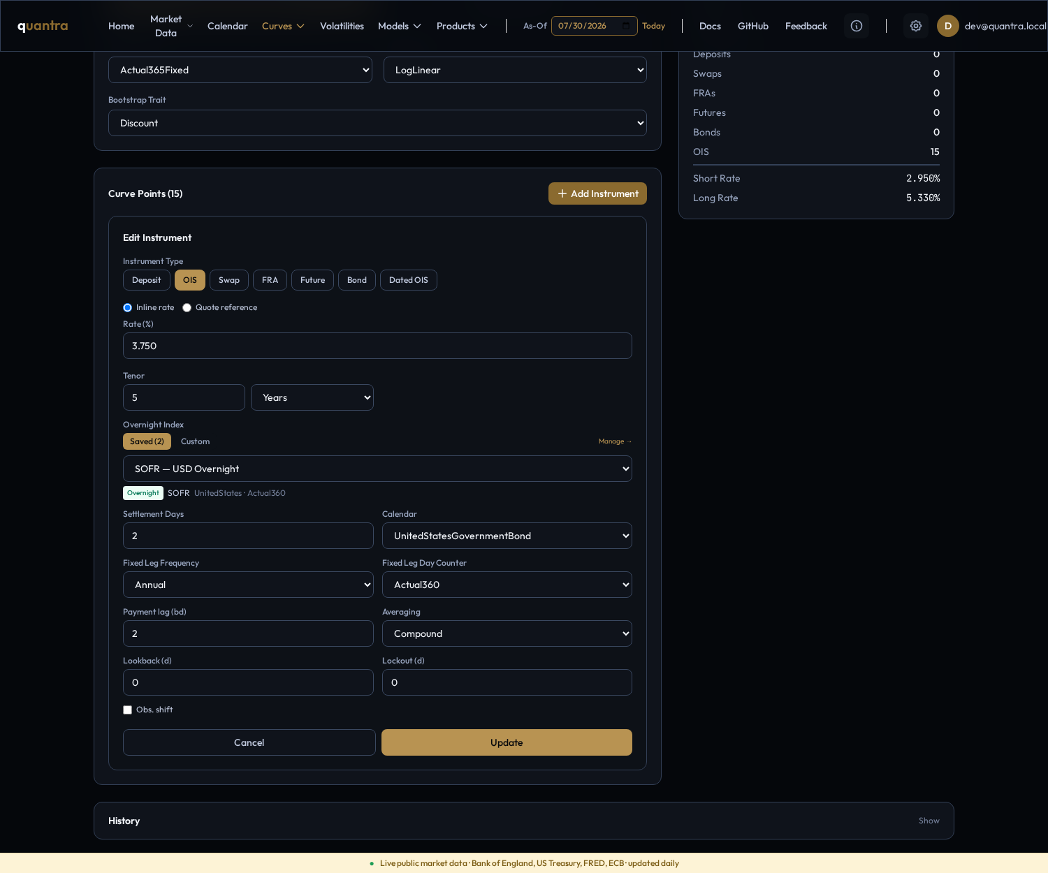
In the portal: Curves, New Yield Curve, construction "Bootstrap from instruments", day counter Actual/365 Fixed, interpolation LogLinear, trait Discount. Then one OIS instrument per quote. The OIS instrument form takes the quote and tenor, the overnight index, settlement days, the fixed leg conventions, and the overnight parameters: payment lag, averaging (Compound or Simple), lookback days, lockout days and the observation shift flag.
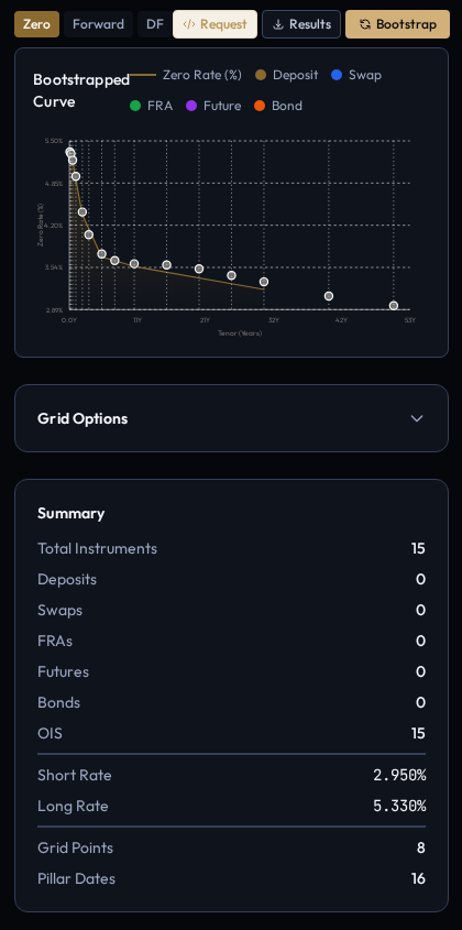
Setting the tenor grid to run out to 50 years and pressing Bootstrap returns the discount factors and zero rates on the grid; the bootstrapped zeros run from 5.39% at one month down to 2.67% at fifty years.
These parameters need pricing engine 0.6.0 or later; on older engines the OIS helpers do not carry them and the request is rejected. Both curves from this post are saved on the public demo as "USD SOFR OIS example (payment lag 2)" and "(payment lag 0)": open either under Curves, press Bootstrap, and compare the long end yourself.
The same call to the engine
The engine is its own open source project with a plain JSON API, and the portal produces exactly this request. The market data block defines the index and the curve; abridged to one helper, with every parameter from the walk above visible on the wire:
{
  "pricing": {
    "as_of_date": "2025-01-15",
    "rates": {
      "indices": [{
        "id": "USD_SOFR", "name": "SOFR", "index_type": "Overnight",
        "currency": "USD", "tenor": {"n": 0, "unit": "Days"},
        "fixing_days": 0, "calendar": "UnitedStatesGovernmentBond",
        "day_counter": "Actual360",
        "business_day_convention": "ModifiedFollowing", "end_of_month": true
      }],
      "curves": [{
        "id": "USD_SOFR_OIS", "reference_date": "2025-01-15",
        "day_counter": "Actual365Fixed", "interpolator": "LogLinear",
        "bootstrap_trait": "Discount",
        "points": [
          {"point_type": "OISHelper", "point": {
            "rate": 0.0375, "tenor": {"n": 5, "unit": "Years"},
            "overnight_index": {"id": "USD_SOFR"}, "settlement_days": 2,
            "calendar": "UnitedStatesGovernmentBond",
            "fixed_leg_frequency": "Annual",
            "fixed_leg_convention": "ModifiedFollowing",
            "payment_lag": 2, "averaging_method": "Compound",
            "lookback_days": 0, "lockout_days": 0,
            "apply_observation_shift": false
          }}
        ]
      }]
    }
  },
  "queries": [{
    "curve_id": "USD_SOFR_OIS", "measures": ["DF", "ZERO"],
    "grid": {"grid_type": "TenorGrid", "grid": {"tenors": [
      {"n": 1, "unit": "Months"}, {"n": 5, "unit": "Years"},
      {"n": 50, "unit": "Years"}]}}
  }]
}
One detail on the index block: end_of_month is required by the schema for
every index definition because the same index shape serves both term and
overnight indices, and the engine requires every convention explicitly rather
than defaulting any of them. For a term index like EURIBOR it decides how month
end maturities roll; for an overnight index it is carried but has no effect,
since maturities are a single day forward rather than a whole number of months.
The complete request with all 15 helpers and the full tenor grid, runnable as
is, is sofr-bootstrap-request.json.
POST /bootstrap-curves with it returns the grid:
{"results": [{"id": "USD_SOFR_OIS", "reference_date": "2025-01-15",
  "grid_dates": ["2025-02-18", "...", "2075-01-15"],
  "series": [
    {"values": [0.994990587471, "...", 0.262755579831]},
    {"measure": "ZERO", "values": [0.053912665272, "...", 0.026713055914]}]}]}
The same curve in QuantLib
QuantLib is the engine's brain, so the check is direct: build the same helpers
with ql.OISRateHelper, bootstrap with the same trait and interpolation, read
the same grid dates. The one mapping worth knowing is where the helper fields
land: the helper's calendar, fixed leg frequency and fixed leg convention feed
QuantLib's payment calendar, payment frequency and payment convention arguments.
import QuantLib as ql

as_of = ql.Date(15, 1, 2025)
ql.Settings.instance().evaluationDate = as_of
cal = ql.UnitedStates(ql.UnitedStates.GovernmentBond)
sofr = ql.Sofr()

quotes = [((1, ql.Months), 0.0533), ((3, ql.Months), 0.0530),
          ((6, ql.Months), 0.0520), ((1, ql.Years), 0.0495),
          ((2, ql.Years), 0.0440), ((3, ql.Years), 0.0405),
          ((5, ql.Years), 0.0375), ((7, ql.Years), 0.0365),
          ((10, ql.Years), 0.0360), ((15, ql.Years), 0.0358),
          ((20, ql.Years), 0.0352), ((25, ql.Years), 0.0342),
          ((30, ql.Years), 0.0332), ((40, ql.Years), 0.0310),
          ((50, ql.Years), 0.0295)]

helpers = [
    ql.OISRateHelper(
        2,                                # settlement days
        ql.Period(*tenor),
        ql.QuoteHandle(ql.SimpleQuote(rate)),
        sofr,
        ql.YieldTermStructureHandle(),    # no exogenous discount curve
        False,                            # telescopic value dates
        2,                                # payment lag
        ql.ModifiedFollowing,             # payment convention
        ql.Annual,                        # payment frequency
        cal,                              # payment calendar
    )
    for tenor, rate in quotes
]

curve = ql.PiecewiseLogLinearDiscount(as_of, helpers, ql.Actual365Fixed())
Discount factors, engine response against QuantLib 1.41:
| Date | Engine DF | QuantLib DF | Diff |
|---|---|---|---|
| 2025-02-18 | 0.994990587471 | 0.994990587470898 | 1.0e-13 |
| 2026-01-15 | 0.952154025624 | 0.952154025624167 | 1.7e-13 |
| 2030-01-15 | 0.830817154298 | 0.830817154297631 | 3.7e-13 |
| 2045-01-17 | 0.499033516800 | 0.499033516799824 | 1.8e-13 |
| 2065-01-15 | 0.315036563467 | 0.315036563466454 | 5.5e-13 |
| 2075-01-15 | 0.262755579831 | 0.262755579830758 | 2.4e-13 |
Largest difference across the grid: 5.5e-13, which is the JSON response's twelve decimal serialization, not the models disagreeing.
Pricing a swap against the curve
The point of the curve is what it prices. A 5 year payer OIS, ten million
notional, paying 3.00% fixed against compounded SOFR, both legs on the
conventions above. To the engine this is POST /price-ois-swap. The full
request has two parts: the same pricing market data block as the bootstrap
call above (index plus the 15 helper curve, unchanged), and the trade. Shown
here with the pricing block collapsed; the complete request, runnable as is,
is sofr-ois-swap-request.json:
{
  "pricing": { "... the market data block from the bootstrap call ..." },
  "swaps": [{
    "ois_swap": {
      "swap_type": "Payer",
      "fixed_leg": {
        "notional": 10000000.0, "rate": 0.03, "day_counter": "Actual360",
        "payment_convention": "ModifiedFollowing",
        "schedule": {
          "calendar": "UnitedStatesGovernmentBond",
          "effective_date": "2025-01-17", "termination_date": "2030-01-17",
          "frequency": "Annual", "convention": "ModifiedFollowing",
          "termination_date_convention": "ModifiedFollowing",
          "date_generation_rule": "Forward", "end_of_month": false}},
      "overnight_leg": {
        "notional": 10000000.0, "index": {"id": "USD_SOFR"}, "spread": 0.0,
        "day_counter": "Actual360", "payment_convention": "ModifiedFollowing",
        "payment_calendar": "UnitedStatesGovernmentBond",
        "payment_lag": 2, "averaging_method": "Compound",
        "lookback_days": 0, "lockout_days": 0,
        "apply_observation_shift": false, "telescopic_value_dates": false,
        "schedule": {
          "calendar": "UnitedStatesGovernmentBond",
          "effective_date": "2025-01-17", "termination_date": "2030-01-17",
          "frequency": "Annual", "convention": "ModifiedFollowing",
          "termination_date_convention": "ModifiedFollowing",
          "date_generation_rule": "Forward", "end_of_month": false}}},
    "discounting_curve": "USD_SOFR_OIS",
    "forwarding_curve": "USD_SOFR_OIS"}]
}
The response:
{"swaps": [{"npv": 337986.79130030936,
            "fair_rate": 0.0375, "fair_spread": -0.0075,
            "fixed_leg_npv": -1351947.1652012337,
            "overnight_leg_npv": 1689933.956501543}]}
Two sanity checks fall out of this. The fair rate is 3.7500%, exactly the 5 year quote in the strip: repricing a calibration instrument at par is what a correct bootstrap means. And paying 3.00% when par is 3.75% has positive value to the payer, about 75 basis points of annuity.
The same swap in QuantLib:
handle = ql.YieldTermStructureHandle(curve)
sofr_fc = ql.Sofr(handle)

schedule = ql.Schedule(
    ql.Date(17, 1, 2025), ql.Date(17, 1, 2030), ql.Period(ql.Annual),
    cal, ql.ModifiedFollowing, ql.ModifiedFollowing,
    ql.DateGeneration.Forward, False)

swap = ql.OvernightIndexedSwap(
    ql.OvernightIndexedSwap.Payer, 10_000_000.0, schedule,
    0.03, ql.Actual360(), sofr_fc,
    0.0,                     # spread
    2,                       # payment lag
    ql.ModifiedFollowing, cal, False)
swap.setPricingEngine(ql.DiscountingSwapEngine(handle))
| NPV | Fair rate | |
|---|---|---|
| Engine | 337986.79130031 | 3.750000000000% |
| QuantLib 1.41 | 337986.79130067 | 3.750000000000% |
A difference of 3.7e-7 dollars on ten million notional.
The engine's JSON API is also public on the demo, so both request files in this post run against it directly:
curl -X POST https://api.quantra.io/price-ois-swap \
  -H "Content-Type: application/json" -d @sofr-ois-swap-request.json
References
- Federal Reserve Bank of New York, Secured Overnight Financing Rate data and the SOFR methodology.
- Alternative Reference Rates Committee, An Updated User's Guide to SOFR (2021): the conventions catalog the lookback, lockout and observation shift definitions come from.
- Ametrano, F. and Bianchetti, M., Everything You Always Wanted to Know About Multiple Interest Rate Curve Bootstrapping but Were Afraid to Ask (2013): the standard reference on modern curve bootstrapping.
- QuantLib, OISRateHelper and the QuantLib Python documentation.